Accuracy (准确率), Precision (精确率), Recall (召回率)
Accurary
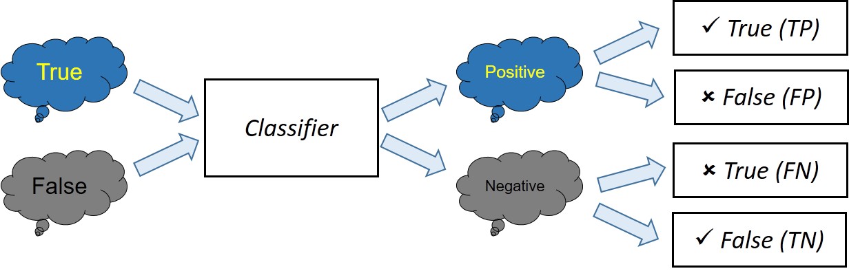
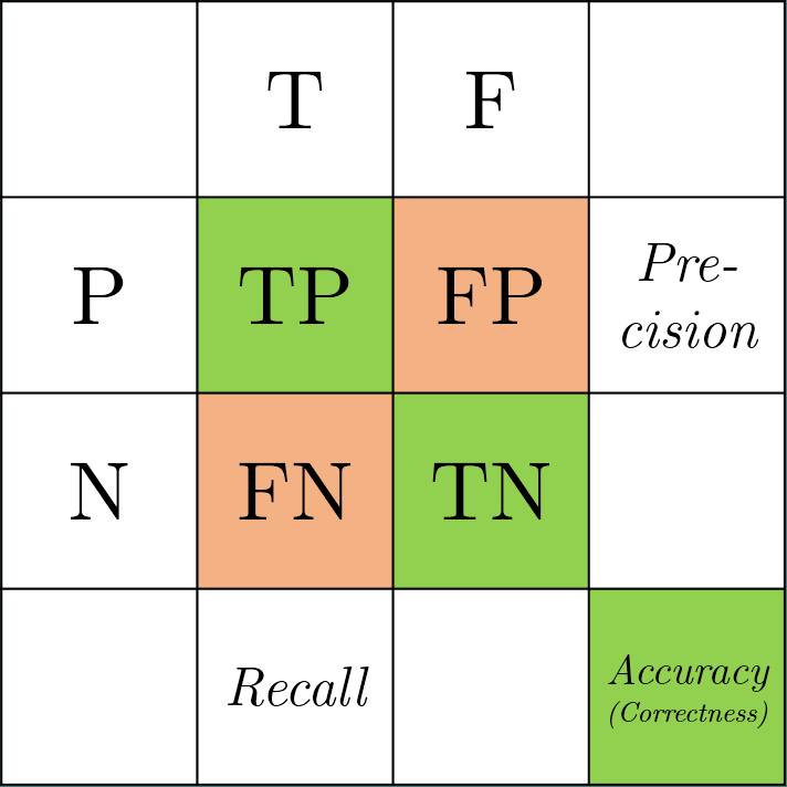
Normally in our model testing, we use accuracy to measure the performance of the model. It calculates the “correctness” of the model.
\[\text{Accuracy} = \text{Correctness} = \frac{TP + TN}{\text{All}} = \frac{TP + TN}{TP + TN + FP + FN}\]Similarly, we also use “Error Rate” to refer $1 - \text{Accuracy}$.
Precision
If we talk about the term “Precision” in machine learning, it refers to the ratio of the number of TP over the number of samples classified as Positive.
\[\text{Precision} = \frac{TP}{P} = \frac{TP}{TP + FP}\]Recall
Recall refers to the ratio of the number of TP over the number of True samples.
\[\text{Recall} = \frac{TP}{T} = \frac{TP}{TP + FN}\]An Example (Original webpage)
假如某个班级有男生80人,女生20人,共计100人.目标是找出所有女生. 现在某人挑选出50个人,其中20人是女生,另外还错误的把30个男生也当作女生挑选出来了. 作为评估者的你需要来评估(evaluation)下他的工作.
Solution:
- 目标:找出所有女生
=>女生:True, 男生:False - $F = 80, T = 20. P = 50, TP = 20, FP = 30$ Since $TP + FN = T$, $FN = T - TP = 20 - 20 = 0$. And $F = FP + TN$, $TN = F - FP = 80 - 30 = 50$.
We can get: $$\begin{align} \text{Precision} & = TP / P = 20 / 50 = 40\% \newline \nonumber \text{Recall} & = TP / T = 20 / 20 = 100\% \newline \nonumber \text{Accuracy} & = (TP + TN) / All = (20 + 50) / 100 = 70\% \newline \nonumber \end{align}$$
Overfitting and Underfitting
Overfitting
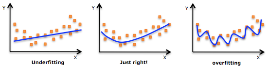
Given a set of data, we use a model to fit it, or say “to train” it. If the parameters of the model are too many, the model will have too much degree-of-freedom, so that the model fits every details of the training data, but loses its generalization to the problem. This case is called “overfitting”.
Two reasons causing overfitting:
- The feature distributions of the training data and validation data are not the identical.
- The model is too complicated as introduced above, but the training samples are not enough.
The solutions to avoid overfitting:
-
Cross validation
Divide the whole training dataset into two parts, saying 90% as training data, and the rest 10% as validation data. We can do multiple training experiments and each time leave one alone, to cross validate the training and validation dataset. This method is to avoid to learn the local features in training dataset.
-
Regularization
Regularization refers to adding more constraints to the original training problem, so that reduce the complexity of the model. For example L1 or L2 norm as regularization, to force the sparsity of parameters.
- More diverse traing samples (data augmentation)
- Collect more data from the original domain;
- Duplicate the existing training data and add noise to them;
- Estimate the data structure of the training data and synthesize more data with the similar structure.
-
Early stopping
Normally if for a continuous several epoches, saying 10, the validation accuracy will not go to a higher accuracy, we think the accuracy will not become better, so we stop the training. The idea is to avoid too much training causing overfitting.
-
Dropout
For neural network, we randomly unconnect some connections between neurons to add some randomness. This may forget some local patterns the model learned which are not applicable to global data.
Underfitting
The same as above, given a set of data, we use a model to fit it. However, this time the parameters of the model are not enough, the model will have limited degree-of-freedom, so that the model cannot well fit the training data. This case is called “underfitting”.
Example to Explain: Black Bird
Saying you need to build a model to recognize birds out of animals. You have a dataset containing lots of birds, they all have wings, feather and occasionally they are all black. And if your model have two much parameters to fit the dataset, it probaby learns that a bird must be black, so that if you input a white bird, even it has wings and feather the classifier won’t recognize it. In this case, we say the classifier has been overfitted.
Now if you model only contains a parameter about feather, it will result in that the model cannot well distinguish birds from chickens. So two few parameters may cause the model too simple to fit the dataset.
K-Means and GMM
For K-Means, $K$ is specified.
Algorithm:
- Initialize $K$ centers ${c_k}$.
- For each data point $x_i$, calculate its distance to the $K$ centers: $d_{i,k}$, choose the nearest center as its group. So that for each center $c_k$, it has a group of data points $x_{i,k}$.
- Update the center position: $c_k = \frac{1}{N_k}\sum_i x_{i,k}$, where $N_k$ is the number of $x_{i,k}$
- Go to Step 2, repeat until $c_k$ only change its position within a threshold.
For GMM, its number of components $K$ is also specified.
GMM is a generative model. Its meaning is: We have a dataset, and we assume that they are generated from a GMM. So for each data point $x$, it should follow the PDF of GMM:
\[p(x|\theta) = \sum_{k = 1}^K p(k)p(x|k) = \sum_{k = 1}^K \pi_k \mathcal{N}(x|\mu_k,\Sigma_k)\]where $\theta$ is all the parameters in the problem: ${\pi_k}, {\mu_k}, {\Sigma_k}$.
Bayesian Theory
\[p(\theta|x) = \frac{p(x|\theta) p(\theta)}{p(x)}\]Data is generated by the parameter.
- Likelihood: \(p(x \vert \theta)\). given parameter, how likely of the data $x$ is generated by the parameter.
- Prior: \(p(\theta)\).
- Posterior: \(p(\theta \vert x)\), meaning that given the data $x$, the conditional density of the parameters.
We need to calculate the maximum likelihood function \(\prod_{i = 1}^N p(x_i \vert \theta)\), apply log to it: \(\sum_{i = 1}^N \log p(x_i \vert \theta)\). Since \(p(x_i \vert \theta)\) contains adding, so it is difficult to calculate the gradient for parameters. So we follow the two steps like in K-Means.
Algorithm:
- Initialize $K$ gaussian distributions, each one has known parameters.
-
(Expectation) For each data point $x_i$, calculate the probability it belongs to $k$-th component (or generated by $k$-th component).
\[\gamma(i, k) = \frac{\pi_k\mathcal{N}(x_i|\mu_k,\Sigma_k)}{\sum_{j = 1}^K\pi_j\mathcal{N}(x_i|\mu_j,\Sigma_j)}\] -
(Maximization) Update the component parameter:
\[\begin{align} \mu_k & = \frac{1}{N_k}\sum_i^N\gamma(i,k)x_i \newline \nonumber \Sigma_k & = \frac{1}{N_k}\sum_i^N\gamma(i,k)(x_i - \mu_k)(x_i - \mu_k)^T \newline \nonumber N_k & = \sum_{i = 1}^N\gamma(i,k), \pi_k = N_k / N \end{align}\]we can interpret that $k$-th component generates $\gamma(i,k)x_i$.
- Go to Step 2, until converge.
Check pluskid’s blog here.

